Running a model
After having built a fratoo model, a wide range of different model runs can be performed.
First, the model, i.e., model equations and input data, has to be loaded (the workflow shown here assumes a Pyomo-based model file is used):
import fratoo as ft

osemosys = "example_model/OSeMOSYS-Pyomo_2019_05_13.py"
data = "example_model/datapackage.json"

model = ft.Model(model=osemosys, data=data, process=True)
Second, the model can be run by defining the names and spatial entities for each run:
names = ["run_1","run_2"]
entities = [[["UK"]],[["Camden"]]]

model.perform_runs(names, entities)
A more detailed description of the perform_runs() method and how it can be used to perform different kind of model runs is given below.
Finally, results can be visualized, for example:
model.plot_capacity(zfilter_str_out="TF",
                    zfilter={"RUN":"Scenario_1"},
                    zgroupby="TECHNOLOGY")
A detailed description of the plot functions is given in the code and some examples are given below.
Defining model runs
As discussed in the introduction, being able to flexibly run different geographic entities of the model while potentially aggregating them or the results is a key feature of fratoo designed to facilitate the creation of scenario pathways and insights relevant across spatial and governance scales.
This is implemented through a flexible perform_runs() method which takes a number of arguments defining the required model runs and saves the results in the results attribute of the model. It has the following core arguments:
names(list): A list of names of the model runs. Model runs can represent, for example, different scenarios for the same spatial entity or runs of different spatial entities.entities(list): A nested list of the spatial entities explicitly included in each run. Each sublist for a single run includes lists of strings where each subsublist contains the names of the regions part of a single optimization and (optional) subsubsublist (sorry) contain entities that are to be aggregated. This is explained in more detail below. It must be the same length asnames.func(list, optional): A list of functions to be applied to the input data set for each of the model runs. The functions take the input data set in form of a dictionary as parameter and return the amended input data dictionary. It must be the same lengths asnames, if given.autoinclude(bool, optional): A boolean argument deciding if the runs are to automatically also include parent and child entities of explicitly listed ones inentities. The default is True.weights(str, optional): Name of the parameter that is used to as weight when calculating the fraction of parent regions. The parameter needs to be defined over the REGION set. If None is given equal weights are assumed. The default is None.processes(int, optional): The number of CPU processes to be used to solve model runs. If it is set higher than the number of model runs, the number of model runs is used instead. The default is 1.join_results(bool, optional): A boolean argument deciding if results of the runs are to be saved in a combined DataFrame. The default is False.overwrite(bool, optional): A boolean argument deciding if previous results, if existing, are to be overwritten. If False, the runs will not proceed if results already exist and a warning is given. The default is False.
The entities arguments for the perform_runs() method is the nested list of entities to be considered for the model runs. A breakdown of the nested list levels is given below based on this example:
entities = [[[["area_1","area_2"],"area_3"]],
            [["area_1"],["area_2","area_4"]]]
The example comprises two model runs, i.e., [[["area_1","area_2"],"area_3"]] and [["area_1"],["area_2","area_4"]].
The first run comprises one optimization, i.e., [["area_1","area_2"],"area_3"] the second run consists of two separate optimizations, i.e., ["area_1"] and ["area_2","area_4"].
The first and only optimization of the first run consists of two explicitly listed entities, i.e., ["area_1","area_2"] (an aggregated area consisting of "area_1" and "area_2") and "area_3". The second run’s two optimizations consist of a single entity, "area_1", and two entities, "area_2" and "area_4", respectively.
While creating the entities list for model runs, it is also important to consider the autoinclude functionality. If autoinclude is set to True (by default, it is), the runs will automatically also include (recursively) parent and child entities of the explicitly listed ones in entities. All child entities on the same scale and with the same explicit parent (i.e., that are included based on the same explicitly listed entity) will be aggregated to a single entity. Parent entities will be disaggregated/only included partially (with the weights attribute definining which parameter is used to calculate the fraction that is included based on which child regions are included) if not all of its child entities are part of the model run. If child entities are to be aggregated, respective parameters will be aggregated based on the rule (e.g., average or sum) given in the input data file ft_param_agg.csv. If parent entities are to be disaggregated, respective parameters will be calculated based on the rule (e.g., equal or fraction) given in the input data file ft_param_disagg.csv. The examples below illustrate this autoinclude functionality.
Examples
Following examples are to illustrate the use of the perform_runs() function. The figure below shows the entities in the multi-scale geography of the example model.
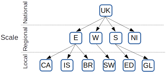
Multi-scale geography with 3 different scales (national, regional, local) and 11 spatial entities: United Kingdom (UK), England (E), Wales (W), Scotland (S), Northern Ireland (NI), Camden (CA), Islington (IS), Brighton (BR), Swansea (SW), Edinburgh (ED), Glasgow (GL).
For example 1, the aim is to develop an aggregated scenario pathway for the entire country but with a focus on a single local area, in this case Camden. This is to be achieved by a performing a two region run: Camden and the rest-of-the-UK. This can be achieved with the following commands:
names = ["Example_1"]
entities = [[["UK","Camden"]]]

model.perform_runs(names, entities)
As can be seen in the figure below, the run includes 4 spatial entities: Camden, the UK, an aggregated entity of all regions, and an aggregated entity of all local areas except Camden.

Multi-scale geography for the run of example 1: the UK and Camden are included as explicitly listed entities (red), while the others are included as (grand)child entities (orange) of the UK.
In contrast, example 2 aims to develop an aggregated scenario pathway only for England:
names = ["Example_2"]
entities = [[["England"]]]

model.perform_runs(names, entities)
As can be seen in the figure below, the run includes 3 spatial entities: an aggregated entity of all local areas in England, England, and the (partial) UK.

Multi-scale geography for the run of example 2: England is included as explicitly listed entity (red), the UK as the parent entity of England (green) and local areas as child entities of England (orange). The greyed out entities are not considered for the run.
Example 3 shows how a single run can consist of several optimizations. Its aim is to establish a scenario pathway for the entire UK with detailed knowledge about pathways in each local area. Assuming that running a single optimization with all entities is computationally not tractable, each local area is optimized separately and results are aggregated.
names = ["Example_3"]

entities = [[["Camden"],["Islington"],["Brighton"],
             ["Swansea"],["Edinburgh"],["Glasgow"]]]

model.perform_runs(names, entities)
The figure below shows exemplarily the entities part of the first optimization looking at Camden. It includes 3 spatial entities: Camden, (partial) England, and the (partial) UK. After solving all optimizations, the results will be aggregated.
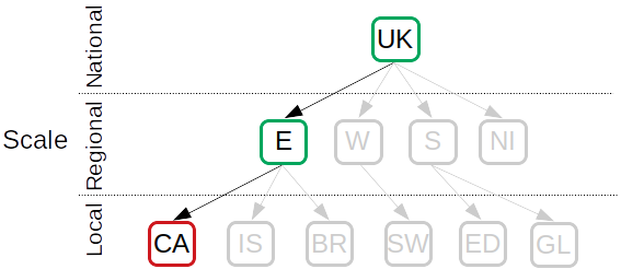
Multi-scale geography for the first optimization of the run of example 3: Camden is included as explicitly listed entity (red) and England and the UK as the (grand) parent entities of Camden (green). The greyed out entities are not considered for the optimization.
Example 4 shows how to run different scenarios by changing input data. For this example, scenario pathways for Camden and Islington, as one aggregated entity, are to be established for two different scenarios: the Base scenario and the PV scenario, in which the capital cost of photovoltaic (PV) panels is lower.
def base(d):
    d["CapitalCost"][d["CapitalCost"].index.get_level_values("TECHNOLOGY")=="PV"] = 1000
    return d
def PV(d):
    d["CapitalCost"][d["CapitalCost"].index.get_level_values("TECHNOLOGY")=="PV"] = 500
    return d

names = ["Base","PV"]
entities = [[[["Camden","Islington"]]],
            [[["Camden","Islington"]]]]
functions = [base, PV]


model.perform_runs(names, entities, functions)
As can be seen above, the input data dictionary passed to the scenario functions consists of the parameter names as the keys and Pandas DataFrames of the actual data as the respective values.
The figure below shows the entities part of each of the runs. It includes 3 spatial entities: an aggregated area of Camden and Islington, (partial) England, and the (partial) UK.
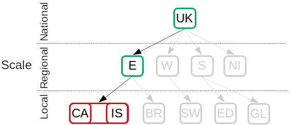
Multi-scale geography for both runs of example 4: an aggregated entity for Camden and Islington is included as explicitly listed entity (red) and England and the UK as the (grand) parent entities (green). The greyed out entities are not considered for these runs.
Visualizing results
fratoo provides a few flexible plotting functions for a quick analysis of model runs. For more specialized plots, results data can be accessed through the results dictionary and plotted manually in Python or otherwise, e.g., in a spreadsheet.
There are two main plotting methods, plot_results() for graphs and plot_map() for maps. Moreover, two methods that use the former are introduced to quickly plot standard graphs, i.e., plot_capacity() and plot_generation(). Some examples are shown below.
plot_results() can be used to look at the activity levels of technologies in different time slices:
model.plot_results("RateOfTotalActivity", x="TIMESLICE",
                    zfilter={"RUN":"Scenario_1","YEAR":2050},
                    zgroupby="TECHNOLOGY", zfilter_str_out="TF",
                    xlabel="Time slice", ylabel="Generation (PJ/a)",
                    kind="bar")
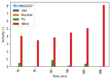
Plot for example 1.
plot_generation() can be used to quickly plot generation time series:
model.plot_generation(zfilter_str_out="TF",
                      zfilter={"RUN":"Scenario_1"},
                      zgroupby="REGION")
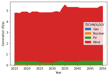
Plot for example 2.
plot_capacity() can be used to quickly plot capacity time series:
model.plot_capacity(zfilter_str_out="TF",
                    zfilter={"RUN":"Scenario_1"},
                    zgroupby="TECHNOLOGY")
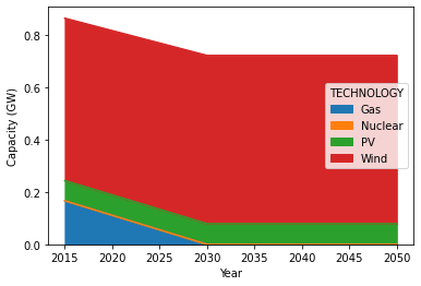
Plot for example 3.
plot_map() can be used to illustrate, e.g., capacity data using maps:
file = "./example_shapefile.shp"

model.plot_map(var="TotalCapacityAnnual",
               zfilter={"TECHNOLOGY":"PV","YEAR":2050},
               mapfile=file, map_column="AREA_ID",
               zlabel="Capacity (GW)")
[Example plot for map to be added]